Tue 07th Jul 2026
Understanding time complexity with sorting algorithms
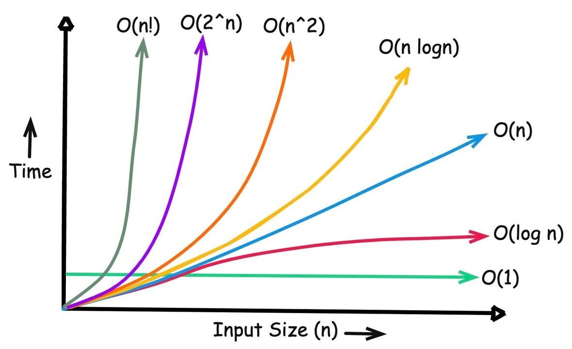
Time complexity in Computer Science is a concept to measure the runtime of an algorithm as input size increases. I delve into the Big O notation and look at how sorting algorithms are classified under the notation in this blog.
Time complexity is a concept in computer science that measures how the runtime of an algorithm grows as the size of the input increases. This is helpful when gauging the performance of an algorithm or a block of code at scale.
At the first time I came across this concept I thought it was actual seconds a computer takes but then later on I came to understand it is the number of basic operations the code has to perform.
Big O Notation
To express time complexity, we use Big O notation, which gives a worst-case scenario of how an algorithm scales. The N represents the size of the input data.
Here are the most common time complexities you'll encounter, ranked from fastest to slowest:
1. Constant Time: O(1)
The execution time stays exactly the same, no matter how huge the input is.
2. Logarithmic Time: O(log N)
The execution time grows, but it slows down drastically the larger the data gets. This usually happens when the algorithm cuts the problem size in half at each step.
3. Linear Time: O(N)
The execution time grows in direct, 1-to-1 proportion with the input size. If you double the data, it takes double the time.
4. Quadratic Time: O(N^2)
The performance depends on the square of the input size. This typically happens when you nest loops inside each other. If your input is 10, it takes 100 steps. If it's 1,000, it takes 1,000,000 steps.
5. Exponential Time: O(2^2) or O(2^N)
The growth doubles with each addition to the input dataset. Algorithms with this complexity quickly become impossible to run for even moderately sized inputs.
So to gauge where you’d want performance to be I think this reddit post gives an accurate description of the notations
Diving deeper using sorting algorithms
Sorting algorithms are one of the best ways to see how time complexity plays out in practice. Because different algorithms use different strategies to organize data, their efficiencies vary wildly.
Here is how sorting algorithms map across the spectrum of time complexity, ordered from the most efficient to the least efficient (in their average or worst-case scenarios).
1. Logarithmic-Linear Time: O(N log N)
While there isn't a standard sorting algorithm that can sort an arbitrary, unsorted list in Constant O(1) or Linear O(N) time, O(N log N) is the gold standard for general-purpose sorting. It represents a "divide-and-conquer" approach.
Merge Sort
- How it works: It recursively splits the unsorted list in half until it has sublists containing exactly one element. Then, it repeatedly merges those sublists back together in the correct order.
- Why it's
O(N log N): Splitting the list in half takes logarithmic time (O(log N)), and merging the elements back together requires looking at every item (O(N)). Combined, they yieldO(N log N). - Performance: Excellent. It performs reliably well regardless of how scrambled the initial data is.
2. Quadratic Time: O(N^2)
Algorithms in this category generally use a brute-force approach, comparing almost every element to every other element.
Bubble Sort
- How it works: It steps through the list, compares adjacent elements, and swaps them if they are in the wrong order. This pass through the list is repeated until no swaps are needed, causing the largest elements to "bubble" to the top.
- Why it's
O(N^2): For a list of sizeN, you have to loop through the list roughlyNtimes, and during each loop, you make roughlyNcomparisons. This nesting of actions results inN times N = N^2operations. - Performance: Poor. If you double the size of your list, Bubble Sort will take four times longer to finish.
Selection Sort
- How it works: It divides the list into a sorted part and an unsorted part. It repeatedly finds the smallest (or largest) element in the unsorted part and moves it to the end of the sorted part.
- Why it's
O(N^2): Like Bubble Sort, it relies on nested loops to scan the remaining unsorted elements of the array to find the minimum value. - Performance: Poor. It performs the same sluggish number of operations even if the array is already mostly sorted.
3. Exponential Time: O(2^N)
True exponential sorting algorithms are rare in practice because they are incredibly inefficient, but they can occur when using highly flawed recursive strategies.
Recursive Bubble Sort (Without Optimization)
- How it works: Imagine a recursive algorithm where to sort a list of size
N, the function spawns multiple redundant recursive calls to sort sub-segments of the data without remembering what it has already sorted. - Why it's
O(2^N): If every single step of the algorithm branches out into two or more new sorting operations, the total number of operations doubles with every single element you add to the array. - Performance: Terrible. Sorting a mere 40 items could require over a trillion operations.
4. Combinatorial / Factorial Time: O(N!)
Worse than exponential time is factorial time. While not strictly exponential, it represents the absolute worst-case scenario of algorithmic scaling.
Bogosort (Permutation Sort)
- How it works: Bogosort is a joke algorithm based on pure probability. It throws the elements of the list into the air, lets them land randomly, and checks if they happen to be sorted. If they aren't, it shuffles them randomly again.
- Why it's
O(N!): Because it generates random permutations, it has to cycle through theN!(N factorial) possible arrangements of the list. - Performance: Unusable. Sorting a deck of 52 cards using Bogosort could theoretically take longer than the lifespan of the universe :)
Resources
https://www.youtube.com/watch?v=D6xkbGLQesk - use this especially to know how the mathematics comes about